// sections-bounce.jsx — Bounce timeline and basin map

const { useState: useStateB, useMemo: useMemoB, useEffect: useEffectB, useRef: useRefB, useCallback: useCallbackB } = React;
const { nearestIdx, viridisColor, fmt: fmtB } = window.ECEM;

// ============== Bounce timeline ==============
function BounceTimeline({ data }) {
  // Parsed bounce_hero.json.
  const [tCursor, setTCursor] = useStateB(0);
  const [playing, setPlaying] = useStateB(false);
  const rafRef = useRefB(null);
  const tCursorRef = useRefB(tCursor);
  useEffectB(() => { tCursorRef.current = tCursor; }, [tCursor]);

  const tMin = data.t[0], tMax = data.t[data.t.length - 1];
  const idx = useMemoB(() => nearestIdx(data.t, tCursor), [tCursor, data.t]);

  // Keep the interactive EoS panel readable by masking the coordinate-singular
  // tail of w_eff before it runs into the frame.
  const Hmax = useMemoB(() => Math.max(...data.H.map(Math.abs)), [data.H]);
  const Hmask = 0.02 * Hmax;
  const rhoBounce = data.rho_b;
  const wDisplayDomain = [-2.0, 0.6];
  const wEffMasked = useMemoB(() => data.w_eff.map((v, i) => {
    if (Math.abs(data.H[i]) < Hmask) return NaN;
    const pad = 0.04 * (wDisplayDomain[1] - wDisplayDomain[0]);
    if (!Number.isFinite(v) || v < wDisplayDomain[0] + pad || v > wDisplayDomain[1] - pad) return NaN;
    return v;
  }), [data.w_eff, data.H, Hmask]);

  // Friedmann constraint residual: R(t) = H^2 - (rho_tot - rho_s)/3.
  // Should stay close to zero throughout if the integration is faithful.
  const residual = useMemoB(() => {
    return data.H.map((H, i) => H * H - (data.rho_tot[i] - data.rho_s[i]) / 3.0);
  }, [data.H, data.rho_tot, data.rho_s]);
  const residualAbsMax = useMemoB(() => Math.max(...residual.map(Math.abs)), [residual]);
  const residualDomain = [-residualAbsMax * 1.15, residualAbsMax * 1.15];

  useEffectB(() => {
    if (!playing) return;
    let last = performance.now();
    const tick = (now) => {
      const dt = (now - last) / 1000;
      last = now;
      let next = tCursorRef.current + dt * 1.5; // playback speed
      if (next > tMax) next = tMin;
      tCursorRef.current = next;
      setTCursor(next);
      rafRef.current = requestAnimationFrame(tick);
    };
    rafRef.current = requestAnimationFrame(tick);
    return () => cancelAnimationFrame(rafRef.current);
  }, [playing, tMin, tMax]);

  // Series for the top panels.
  const aData = { x: data.t, y: data.a };
  const HData = { x: data.t, y: data.H };
  const wTotData = { x: data.t, y: data.w_tot };
  const wEffData = { x: data.t, y: wEffMasked };

  // Density components for the log-scale panel.
  const dSeries = [
    { nameTex: '\\rho_m',        color: 'var(--matter)',   x: data.t, y: data.rho_m },
    { nameTex: '\\rho_s',        color: 'var(--bounce)',   x: data.t, y: data.rho_s, width: 1.8 },
    { nameTex: '\\rho_\\varphi', color: 'var(--scalar)',   x: data.t, y: data.rho_phi.map(v => Math.max(v, 1e-30)) },
    { nameTex: '\\rho_\\sigma',  color: 'var(--shear)',    x: data.t, y: data.rho_sigma },
    { nameTex: '\\rho_{\\rm tot}', color: 'var(--ink)',    x: data.t, y: data.rho_tot, width: 1.6 },
  ];

  // Density-domain bounds for the log plot.
  const dMin = 1e-12, dMax = Math.max(...data.rho_tot) * 2;

  // Vertical bounds for a(t), H(t), and w_eff(t).
  const aMax = Math.max(...data.a);

  const cursorOpt = { vLines: [{ x: tCursor, color: 'var(--ekpyrotic)', width: 1.2, dash: '4 3' }] };

  const cur = {
    t: data.t[idx], a: data.a[idx], H: data.H[idx],
    rho_tot: data.rho_tot[idx], rho_s: data.rho_s[idx], rho_m: data.rho_m[idx], rho_phi: data.rho_phi[idx],
    w_eff: data.w_eff[idx], q: data.q[idx],
  };

  // Dominant component at the cursor.
  const componentsRanked = [
    { kTex: '\\rho_s', v: cur.rho_s, color: 'var(--bounce)' },
    { kTex: '\\rho_m', v: cur.rho_m, color: 'var(--matter)' },
    { kTex: '\\rho_\\varphi', v: cur.rho_phi, color: 'var(--scalar)' },
  ].sort((a, b) => b.v - a.v);
  const dominant = componentsRanked[0];

  // Simple phase label at the cursor.
  let phaseLabel = 'Contraction';
  if (Math.abs(cur.H) < 0.005 * Math.max(...data.H.map(Math.abs))) phaseLabel = 'Bounce';
  else if (cur.H > 0) phaseLabel = 'Expansion';

  return (
    <section id="bounce" className="figure col-wide">
      <div className="figure-head">
        <div>
          <span className="label">Figure 4</span>
          <div className="title">Torsion-regulated Einstein-Cartan bounce</div>
        </div>
        <span className="meta"><M tex="k=0" />{' '}benchmark · Radau</span>
      </div>

      <div className="figure-body">
        <div className="journal-pair">
          <figure>
            <img className="journal-figure-img" src="assets/journal-figures/fig4a-1.png" alt="Published Fig. 4a bounce background diagnostics" />
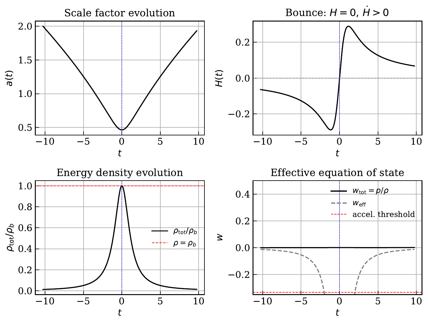
            <figcaption>(a) Background evolution and equation-of-state diagnostics</figcaption>
          </figure>
          <figure>
            <img className="journal-figure-img" src="assets/journal-figures/fig4b-1.png" alt="Published Fig. 4b constraint residual and component densities" />
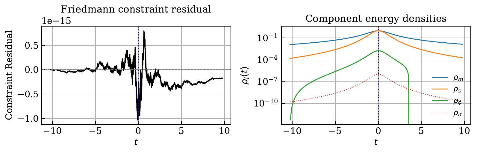
            <figcaption>(b) Friedmann residual and component densities</figcaption>
          </figure>
        </div>
      </div>

      <div className="controls" style={{ justifyContent: 'space-between' }}>
        <span className="eyebrow">Interactive companion</span>
        <span className="meta"><M tex="\varphi_b=0,\,\Delta=0.05,\,\rho_{m,0}=0.1,\,\alpha=10^{-2}" /></span>
      </div>

      <div className="figure-body">
        <div className="timeline-grid">
          {/* (a) scale factor */}
          <div className="panel">
            <h4><M tex="a(t)" /> · scale factor</h4>
            <MultiLinePlot
              series={[{ ...aData, color: 'var(--ink)' }]}
              width={500} height={200}
              xDomain={[tMin, tMax]} yDomain={[0, aMax * 1.05]}
              xLabel="t" yLabel="a"
              vLines={cursorOpt.vLines}
              highlightIdx={idx}
            />
          </div>
          {/* (b) Hubble */}
          <div className="panel">
            <h4><M tex="H(t)" /> · Hubble parameter</h4>
            <MultiLinePlot
              series={[{ ...HData, color: 'var(--bounce)' }]}
              width={500} height={200}
              xDomain={[tMin, tMax]} yDomain={[-Hmax * 1.05, Hmax * 1.05]}
              xLabel="t" yLabel="H"
              hLines={[{ y: 0, color: 'var(--ink-faint)', dash: '4 3' }]}
              vLines={cursorOpt.vLines}
              highlightIdx={idx}
            />
          </div>
          {/* (c) densities log */}
          <div className="panel">
            <h4><M tex="\rho_i(t)" /> · component densities (log)</h4>
            <MultiLinePlot
              series={dSeries}
              width={500} height={200}
              xDomain={[tMin, tMax]} yDomain={[dMin, dMax]}
              yLog
              xLabel="t" yLabel="ρ"
              yFmt={(v) => {
                const e = Math.log10(v);
                return Math.abs(e - Math.round(e)) < 0.01 ? `10${supSign(Math.round(e))}` : '';
              }}
              vLines={cursorOpt.vLines}
              highlightIdx={idx}
            />
            <div className="legend" style={{ padding: '8px 0 0 0' }}>
              {dSeries.map(s => (
                <span key={s.nameTex} className="swatch" style={{ color: s.color }}>
                  <span className="dot" /> <span style={{ color: 'var(--ink-mid)' }}><M tex={s.nameTex} /></span>
                </span>
              ))}
            </div>
          </div>
          {/* (d) w_eff */}
          <div className="panel">
            <h4><M tex="w(t)" /> · equation of state</h4>
            <MultiLinePlot
              series={[
                { ...wTotData, color: 'var(--ink)', width: 1.6 },
                { ...wEffData, color: 'var(--ekpyrotic)', width: 1.4, dash: '5 3' },
              ]}
              width={500} height={220}
              xDomain={[tMin, tMax]} yDomain={wDisplayDomain}
              xLabel="t" yLabel="w"
              hLines={[
                { y: -1/3, color: 'var(--ink-faint)', dash: '4 3' },
                { y: 0, color: 'var(--rule)', dash: '2 2' },
              ]}
              vLines={cursorOpt.vLines}
              highlightIdx={Math.abs(data.H[idx]) < Hmask ? null : idx}
            />
            <div className="legend" style={{ padding: '8px 0 0 0' }}>
              <span className="swatch" style={{ color: 'var(--ink)' }}><span className="dot" /> <span style={{ color: 'var(--ink-mid)' }}><M tex="w_{\rm tot} = \dfrac{p}{\rho}" /></span></span>
              <span className="swatch" style={{ color: 'var(--ekpyrotic)' }}><span className="dot" style={{ background: 'repeating-linear-gradient(90deg, currentColor 0 3px, transparent 3px 5px)' }} /> <span style={{ color: 'var(--ink-mid)' }}><M tex="w_{\rm eff}" />{' '}diverges at{' '}<M tex="H = 0" /></span></span>
            </div>
          </div>
          {/* (e) constraint residual — spans both columns */}
          <div className="panel" style={{ gridColumn: '1 / -1' }}>
            <h4><M tex="\mathcal{R}(t) = H^2 - (\rho_{\rm tot} - \rho_s)/3" /> · Friedmann constraint residual</h4>
            <MultiLinePlot
              series={[{ x: data.t, y: residual, color: 'var(--ink)', width: 1.4 }]}
              width={1000} height={170}
              xDomain={[tMin, tMax]}
              yDomain={residualDomain}
              xLabel="t" yLabel="ℛ"
              hLines={[{ y: 0, color: 'var(--ink-faint)', dash: '4 3' }]}
              vLines={cursorOpt.vLines}
              highlightIdx={idx}
            />
            <div style={{ marginTop: 6, fontSize: 11, color: 'var(--ink-soft)', lineHeight: 1.5 }}>
              The constraint{' '}<M tex="\mathcal{R}" />{' '}is what the Friedmann equation requires to vanish; any drift away is numerical error. Peak excursion here is{' '}<span className="mono" style={{ color: 'var(--ink)' }}>{residualAbsMax.toExponential(2)}</span>, well within the expected range for a Radau integration at the chosen tolerances. The bounce is not an artifact of constraint drift.
            </div>
          </div>
        </div>
      </div>

      <div className="scrubber">
        <button className="play" onClick={() => setPlaying(p => !p)} aria-label={playing ? 'pause' : 'play'}>
          {playing ? '❚❚' : '▶'}
        </button>
        <input type="range" min={tMin} max={tMax} step={(tMax - tMin) / 1000}
          value={tCursor} onChange={e => setTCursor(+e.target.value)} />
        <span className="t-readout">t = {tCursor >= 0 ? '+' : ''}{tCursor.toFixed(2)}</span>
      </div>

      <div className="figure-body metric-grid">
        <div>
          <div className="eyebrow" style={{ fontSize: 9 }}>Phase</div>
          <div style={{ fontSize: 20, marginTop: 4, color: phaseLabel === 'Bounce' ? 'var(--bounce)' : 'var(--ink)' }}>{phaseLabel}</div>
        </div>
        <div>
          <div className="eyebrow" style={{ fontSize: 9 }}>Dominant component</div>
          <div className="mono" style={{ fontSize: 18, marginTop: 4, color: dominant.color }}><M tex={dominant.kTex} /></div>
          <div className="mono" style={{ fontSize: 11, color: 'var(--ink-soft)' }}>{dominant.v.toExponential(2)}</div>
        </div>
        <div>
          <div className="eyebrow" style={{ fontSize: 9 }}><M tex="\dfrac{a}{a_b}" /></div>
          <div className="mono" style={{ fontSize: 18, marginTop: 4 }}>{cur.a.toFixed(3)}</div>
        </div>
        <div>
          <div className="eyebrow" style={{ fontSize: 9 }}><M tex="H" /></div>
          <div className="mono" style={{ fontSize: 18, marginTop: 4 }}>{cur.H >= 0 ? '+' : ''}{cur.H.toExponential(2)}</div>
        </div>
        <div>
          <div className="eyebrow" style={{ fontSize: 9 }}><M tex="\dfrac{\rho_{\rm tot}}{\rho_b}" /></div>
          <div className="mono" style={{ fontSize: 18, marginTop: 4 }}>{(cur.rho_tot / rhoBounce).toFixed(3)}</div>
        </div>
        <div>
          <div className="eyebrow" style={{ fontSize: 9 }}><M tex="w_{\rm tot}" /></div>
          <div className="mono" style={{ fontSize: 18, marginTop: 4 }}>{data.w_tot[idx].toFixed(3)}</div>
          <div className="mono" style={{ fontSize: 10, color: 'var(--ink-soft)', marginTop: 2 }}>
            <M tex="w_{\rm eff}" />: {Math.abs(data.H[idx]) < Hmask ? '—' : cur.w_eff.toFixed(3)}
          </div>
        </div>
      </div>

      <div className="figure-caption">
        <strong>Fig. 4.</strong> Spatially flat{' '}<M tex="k=0" lead="(" tail=")" /> Einstein–Cartan bounce benchmark, integrated with an implicit Radau solver through the stiff{' '}<M tex="H \approx 0" />{' '}region. The universe contracts from a dust-dominated phase until the spin–torsion density matches{' '}<M tex="\rho_{\rm tot}" tail="," /> at which point{' '}<M tex="H=0" />{' '}and{' '}<M tex="\dot H>0" />, giving a nonsingular bounce at a finite scale factor. The effective equation of state{' '}<M tex="w_{\rm eff} = -1 - 2\dot H/(3H^2)" />{' '}is plotted alongside{' '}<M tex="w_{\rm tot} = p/\rho" />; it is masked near{' '}<M tex="H = 0" />{' '}where the definition diverges by construction.
      </div>
    </section>
  );
}

function supSign(n) {
  const sup = { '-': '⁻', '0': '⁰', '1': '¹', '2': '²', '3': '³', '4': '⁴', '5': '⁵', '6': '⁶', '7': '⁷', '8': '⁸', '9': '⁹' };
  return String(n).split('').map(c => sup[c] || c).join('');
}

// ============== Softening-potential mini-plot ==============
// V(phi) = -V0 e^{-lam0 phi} [1 - S(phi)] + V_soft S(phi),
// with S(phi) = (1/2)[1 + tanh((phi - phi_b)/Delta)].
// Draw the potential for one (phi_b, Delta) cell in the basin map.
function PotentialMini({ phi_b, Delta, width = 280, height = 140 }) {
  const V0 = 1e-5, V_SOFT = 1e-5, LAM0 = 3.0;
  const margin = { top: 12, right: 10, bottom: 28, left: 40 };
  const px0 = margin.left, px1 = width - margin.right;
  const py0 = height - margin.bottom, py1 = margin.top;

  // Adapt the phi-window to the transition width so narrow and wide tanh
  // switches both look proportionate.
  const span = Math.max(0.7, 6 * Delta);
  const xMin = phi_b - span;
  const xMax = phi_b + span;

  // Clip the negative ekpyrotic branch so it does not dominate the frame.
  const yMin = -3 * V_SOFT;
  const yMax = 1.8 * V_SOFT;

  const sx = (phi) => px0 + (phi - xMin) / (xMax - xMin) * (px1 - px0);
  const sy = (V) => py0 - (V - yMin) / (yMax - yMin) * (py0 - py1);

  const npts = 240;
  let d = '';
  for (let i = 0; i <= npts; i++) {
    const phi = xMin + (xMax - xMin) * i / npts;
    const S = 0.5 * (1 + Math.tanh((phi - phi_b) / Delta));
    const V = -V0 * Math.exp(-LAM0 * phi) * (1 - S) + V_SOFT * S;
    const Vc = Math.max(yMin, Math.min(yMax, V));
    d += (i === 0 ? 'M' : 'L') + sx(phi).toFixed(2) + ',' + sy(Vc).toFixed(2);
  }

  // Translucent band marking the transition width Delta.
  const bandX0 = sx(Math.max(xMin, phi_b - Delta));
  const bandX1 = sx(Math.min(xMax, phi_b + Delta));

  return (
    <svg className="plot-svg" viewBox={`0 0 ${width} ${height}`}
      preserveAspectRatio="xMidYMid meet" style={{ width: '100%', height: 'auto' }}>
      <rect x={bandX0} y={py1} width={Math.max(0, bandX1 - bandX0)} height={py0 - py1}
        fill="var(--bounce)" opacity="0.07" />
      <rect x={px0} y={py1} width={px1 - px0} height={py0 - py1}
        fill="none" stroke="var(--ink-faint)" strokeWidth="0.7" />
      <line x1={px0} x2={px1} y1={sy(0)} y2={sy(0)}
        stroke="var(--rule)" strokeWidth="0.7" strokeDasharray="2 2" />
      <line x1={sx(phi_b)} x2={sx(phi_b)} y1={py1} y2={py0}
        stroke="var(--bounce)" strokeWidth="1" strokeDasharray="3 2" opacity="0.7" />
      <path d={d} fill="none" stroke="var(--ekpyrotic)" strokeWidth="1.8" />
      <text x={(px0 + px1) / 2} y={height - 8}
        textAnchor="middle" fontSize="10" fill="var(--ink-soft)" fontFamily="var(--font-mono)"><SvgS text="φ" /></text>
      <text x={10} y={(py1 + py0) / 2}
        textAnchor="middle" fontSize="10" fill="var(--ink-soft)" fontFamily="var(--font-mono)"
        transform={`rotate(-90 10 ${(py1 + py0) / 2})`}><SvgS text="V(φ)" /></text>
      <text x={sx(phi_b) + 4} y={py1 + 10}
        fontSize="9" fill="var(--bounce)" fontFamily="var(--font-mono)"><SvgS text="φ_b" /></text>
      <text x={px0} y={py0 + 13}
        fontSize="9" fill="var(--ink-soft)" fontFamily="var(--font-mono)">{xMin.toFixed(1)}</text>
      <text x={px1} y={py0 + 13}
        fontSize="9" fill="var(--ink-soft)" fontFamily="var(--font-mono)" textAnchor="end">{xMax.toFixed(1)}</text>
    </svg>
  );
}

// ============== Basin map ==============
function BasinMap({ basin }) {
  // Basin shape: { phi_b: [], Delta: [], outcome: [], Rb: [], shape: [n_delta, n_phi] }.
  const [hover, setHoverB] = useStateB(null);
  const [selected, setSelected] = useStateB({ i: 10, j: 8 }); // published scan cell

  const ny = basin.shape[0], nx = basin.shape[1];
  // log10(Rb) for cells that bounced.
  const logRb = useMemoB(() => {
    return basin.Rb.map((v, i) => {
      const oc = basin.outcome[i];
      if (oc === 1 && v !== null && v > 0) return Math.log10(v);
      return null;
    });
  }, [basin]);

  const vMin = useMemoB(() => {
    let m = Infinity;
    for (const v of logRb) if (v !== null && v < m) m = v;
    return m;
  }, [logRb]);
  const vMax = useMemoB(() => {
    let m = -Infinity;
    for (const v of logRb) if (v !== null && v > m) m = v;
    return m;
  }, [logRb]);

  const colorScale = useCallbackB((v) => viridisColor((v - vMin) / (vMax - vMin || 1)), [vMin, vMax]);

  // Outcome counts for the header.
  const counts = useMemoB(() => {
    let b = 0, c = 0, u = 0;
    for (const o of basin.outcome) {
      if (o === 1) b++; else if (o === -1) c++; else u++;
    }
    return { b, c, u, total: basin.outcome.length };
  }, [basin]);

  const sel = selected;
  const selV = sel ? logRb[sel.i * nx + sel.j] : null;
  const selOc = sel ? basin.outcome[sel.i * nx + sel.j] : null;
  const selRb = sel ? basin.Rb[sel.i * nx + sel.j] : null;

  const hoverCell = hover || selected;
  const showInfo = hoverCell ? {
    phi_b: basin.phi_b[hoverCell.j],
    Delta: basin.Delta[hoverCell.i],
    v: logRb[hoverCell.i * nx + hoverCell.j],
    Rb: basin.Rb[hoverCell.i * nx + hoverCell.j],
    outcome: basin.outcome[hoverCell.i * nx + hoverCell.j],
  } : null;

  return (
    <section id="basin" className="figure col-wide">
      <div className="figure-head">
        <div>
          <span className="label">Figure 5</span>
          <div className="title">Basin of viability for the softening-spin bounce</div>
        </div>
        <span className="meta">20×20 scan · {counts.b} bounce · {counts.c} crunch · {counts.u} undecided</span>
      </div>
      <div className="figure-body">
        <img
          className="journal-figure-img"
          src="assets/journal-figures/fig5-1.png"
          alt="Published Fig. 5 basin of viability"
        />
      </div>
      <div className="controls" style={{ justifyContent: 'space-between' }}>
        <span className="eyebrow">Interactive companion</span>
        <span className="meta"><M tex="\rho_{m,0}=3\times10^{-4},\,\alpha=10^{-4},\,a_0=3" /></span>
      </div>
      <div className="figure-body">
        <div className="basin-wrap">
          <div className="basin-plot-row">
            <div className="basin-heatmap">
              <Heatmap
                data={logRb}
                xVals={basin.phi_b}
                yVals={basin.Delta}
                outcome={basin.outcome}
                width={560} height={460}
                xLabel="φ_b (softening center)"
                yLabel="Δ (softening width)"
                colorScale={colorScale}
                selected={selected}
                onCellHover={setHoverB}
                onCellClick={({i, j}) => setSelected({i, j})}
              />
            </div>
            <div className="basin-colorbar">
              <svg className="plot-svg" viewBox="0 0 92 460" preserveAspectRatio="xMidYMid meet">
                <ColorbarV
                  colorScale={colorScale}
                  vMin={vMin} vMax={vMax}
                  x={36} y={30} h={320} w={14}
                  label="log_{10} R_b"
                  fmt={(v) => v.toFixed(1)}
                />
              </svg>
            </div>
          </div>
          <div className="basin-sidebar">
            <div className="eyebrow" style={{ fontSize: 9, color: 'var(--ink-faint)' }}>Inspecting</div>
            <div style={{ marginTop: 8 }}>
              <div className="row"><span><M tex="\varphi_b" /></span><span className="v">{showInfo ? showInfo.phi_b.toFixed(2) : '—'}</span></div>
              <div className="row"><span><M tex="\Delta" /></span><span className="v">{showInfo ? showInfo.Delta.toFixed(3) : '—'}</span></div>
              <div className="row"><span><M tex="R_b" /></span><span className="v">{showInfo && showInfo.Rb !== null ? showInfo.Rb.toExponential(2) : '—'}</span></div>
              <div className="row"><span><M tex="\log_{10} R_b" /></span><span className="v">{showInfo && showInfo.v !== null ? showInfo.v.toFixed(2) : '—'}</span></div>
            </div>
            {showInfo && (
              <div className={'verdict ' + (showInfo.outcome === 1 ? 'bounce' : showInfo.outcome === -1 ? 'crunch' : 'undecided')}>
                {showInfo.outcome === 1 ? 'Bounce' : showInfo.outcome === -1 ? 'Crunch' : 'Undecided'}
              </div>
            )}
            {showInfo && (
              <div style={{ marginTop: 16 }}>
                <div className="eyebrow" style={{ fontSize: 9, color: 'var(--ink-faint)', marginBottom: 6 }}>
                  Potential shape for this cell
                </div>
                <PotentialMini phi_b={showInfo.phi_b} Delta={showInfo.Delta} />
                <div style={{ marginTop: 4, fontSize: 11, color: 'var(--ink-soft)', lineHeight: 1.5 }}>
                  Negative ekpyrotic branch on the left, positive plateau on the right, tanh transition of width{' '}<M tex="\Delta" />{' '}centered at the dashed line at{' '}<M tex="\varphi_b" tail="." /> Whether a cell bounces or crunches depends on whether this transition lands close to the density scale where{' '}<M tex="\rho_s" />{' '}catches the scalar.
                </div>
              </div>
            )}
            <div style={{ marginTop: 16, fontSize: 11, color: 'var(--ink-soft)', lineHeight: 1.5 }}>
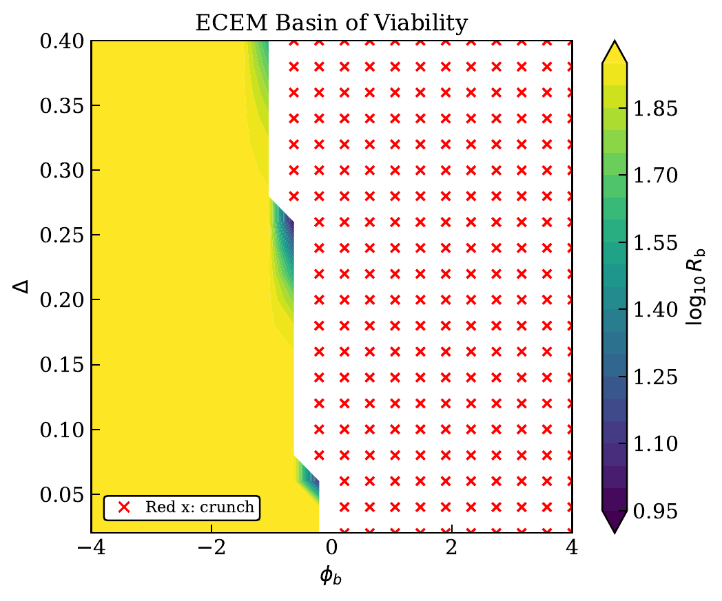
              Red × marks cells where the universe contracted to{' '}<M tex="a \leq 10^{-2}" />{' '}without bouncing (a crunch). Colored cells bounced; the color shows{' '}<M tex="R_b = \rho_s/\rho_\varphi" />{' '}at the moment{' '}<M tex="H = 0" tail="." /> When{' '}<M tex="R_b \gg 1" />{' '}the spin–torsion sector dominates at the bounce; when{' '}<M tex="R_b \sim 1" />{' '}the spin and scalar terms are comparable and the bounce is more marginal.
            </div>
          </div>
        </div>
      </div>
      <div className="figure-caption">
        <strong>Fig. 5.</strong> Bounce basin in the softening-parameter plane{' '}<M tex="(\varphi_b, \Delta)" />{' '}for fixed spin parameter{' '}<M tex="\alpha = 10^{-4}" tail="," /> matter density{' '}<M tex="\rho_{m,0} = 3\times10^{-4}" tail="," /> and initial scale factor{' '}<M tex="a_0 = 3" tail="." /> Each cell is a full integration of the EC system; the white curve is the numerically determined bounce/crunch boundary, which tracks the analytic estimate{' '}<M tex="R_b \approx 1" />{' '}closely. Of the {counts.b + counts.c} trajectories on this grid, {counts.b} bounce and {counts.c} crunch, marking out a finite, tuned but extended region of parameter space.
      </div>
    </section>
  );
}

Object.assign(window, { BounceTimeline, BasinMap });