// sections-close.jsx — Lyapunov panel and closing notes

const { useState: useStateC } = React;

function LyapunovPanel({ data }) {
  // Array of { label, lam, gamma_m, ic, N, lambda_max, final_lambda }.
  const [selected, setSelectedC] = useStateC(0);

  const sel = data[selected];
  const series = [{ x: sel.N, y: sel.lambda_max, color: 'var(--bounce)', width: 1.8 }];

  // Vertical bounds for the selected Lyapunov trace.
  const ymax = Math.max(...sel.lambda_max);
  const ymin = Math.min(...sel.lambda_max);
  const pad = (ymax - ymin) * 0.15 || 0.1;

  return (
    <section id="lyapunov" className="figure col-wide">
      <div className="figure-head">
        <div>
          <span className="label">Figure 2</span>
          <div className="title">Running maximal Lyapunov exponent</div>
        </div>
        <span className="meta">Benettin · 5D constrained · <M tex="\delta_0 = 10^{-8}" /></span>
      </div>
      <div className="figure-body">
        <img
          className="journal-figure-img"
          src="assets/journal-figures/fig2-1.png"
          alt="Published Fig. 2 running maximal Lyapunov exponent panels"
        />
      </div>
      <div className="figure-body lyapunov-companion-grid">
        <div>
          <h4>Interactive readout</h4>
          <MultiLinePlot
            series={series}
            width={560} height={300}
            xDomain={[sel.N[0], sel.N[sel.N.length - 1]]}
            yDomain={[Math.min(0, ymin) - pad, Math.max(0.1, ymax + pad)]}
            xLabel="N (e-fold time)"
            yLabel="running λ_{max}"
            hLines={[{ y: 0, color: 'var(--ink-faint)', dash: '4 3' }]}
          />
        </div>
        <div>
          <h4 style={{ marginTop: 0 }}>Cases</h4>
          <div style={{ display: 'flex', flexDirection: 'column', gap: 8 }}>
            {data.map((c, i) => (
              <button key={i} className={'btn ghost lyapunov-case-btn ' + (i === selected ? 'active' : '')}
                style={{ textAlign: 'left', fontSize: 11, padding: '10px 12px' }}
                onClick={() => setSelectedC(i)}>
                <div style={{ display: 'flex', justifyContent: 'space-between', alignItems: 'baseline', gap: 8 }}>
                  <span>{c.label} <M tex={`\\lambda = ${c.lam},\\, \\gamma_m = ${+(c.gamma_m).toFixed(3)}`} /></span>
                  <span style={{ color: c.final_lambda < 0 ? 'var(--matter)' : 'var(--ekpyrotic)', fontSize: 10 }}>
                    <M tex={`\\lambda_{\\max} \\to ${c.final_lambda.toFixed(3)}`} />
                  </span>
                </div>
              </button>
            ))}
          </div>
          <div style={{ marginTop: 18, padding: 12, background: 'var(--bg)', borderRadius: 'var(--radius)', fontSize: 11, color: 'var(--ink-soft)', lineHeight: 1.55 }}>
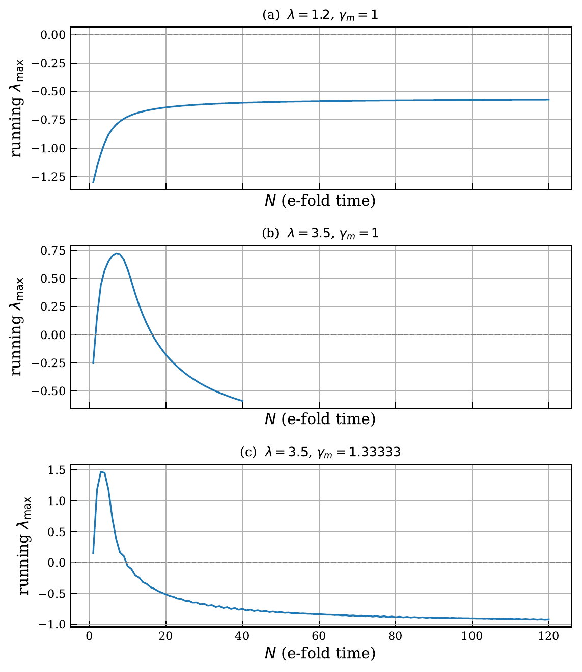
            All three cases settle to a <strong style={{ color: 'var(--matter)' }}>negative</strong> plateau, despite the curvature direction being a growing mode in contracting GR backgrounds. That mode is tied to BKL-type behavior in generic inhomogeneous collapse, so a positive result here would have been important. The homogeneous truncation does not answer what happens once spatial gradients are included, but it does show that the tested phase-space flow on the constraint surface remains ordered.
          </div>
        </div>
      </div>
      <div className="figure-caption">
        <strong>Fig. 2.</strong> Running maximal Lyapunov exponent{' '}<M tex="\lambda_{\max}(N)" />{' '}computed with the Benettin algorithm on the five-dimensional constrained surface (the fluid fraction{' '}<M tex="z" />{' '}is eliminated via the Friedmann constraint). Cases shown:{' '}<M tex="(\lambda,\gamma_m) = (1.2,\,1)" tail="," />{' '}<M tex="(3.5,\,1)" tail="," /> and{' '}<M tex="(3.5,\,4/3)" tail="." /> In each case the exponent settles to a negative plateau on the expanding branch; the early positive excursion in case (b) is a transient, not a sign of chaos.
      </div>
    </section>
  );
}

function Closing() {
  return (
    <section id="closing" className="closing">
      <p>
        <strong style={{ color: 'var(--ink)', fontFamily: 'var(--font-serif)', fontSize: 16 }}>What this paper establishes.</strong>&nbsp;&nbsp;The model is tuned, but within that setup it establishes three concrete results at the homogeneous level. First, ekpyrotic contraction damps shear exponentially before the bounce. The steep negative branch of the potential makes{' '}<M tex="\rho_\varphi" />{' '}grow faster than{' '}<M tex="\rho_\sigma" />{' '}during contraction, so any initial anisotropy decays. Second, a Weyssenhoff spin–torsion sector can replace the would-be singularity with a smooth{' '}<M tex="H = 0" />{' '}crossing where{' '}<M tex="\dot H > 0" tail="," /> at a finite density well below Planckian. Third, the dynamics on the constrained phase space do not show chaos on any tested slice: the maximal Lyapunov exponent stays negative, even with the curvature mode that complicates contracting GR backgrounds. The novelty is not a new microscopic bounce mechanism; it is the global dynamical-systems picture that makes the conditions for a bounce, and the parameter region where one survives, explicit.
      </p>
      <p style={{ marginTop: 18 }}>
        <strong style={{ color: 'var(--ink)', fontFamily: 'var(--font-serif)', fontSize: 16 }}>What it does not claim.</strong>&nbsp;&nbsp;Everything here is a homogeneous background calculation. The model does not address how entropy behaves across cycles, whether the cosmological arrow of time is consistent with repeated bounces, or whether a realistic UV completion of the Weyssenhoff fluid exists. The cycle diagram is a schematic of the four dynamical regimes, not a claim that the universe literally traces a closed orbit in phase space, and it does not answer what happens once spatial gradients (BKL, inhomogeneous mixmaster) are turned on. Those are the questions the next paper would tackle.
      </p>
      <p style={{ marginTop: 18 }}>
        <strong style={{ color: 'var(--ink)', fontFamily: 'var(--font-serif)', fontSize: 16 }}>Numerical notes.</strong>&nbsp;&nbsp;The figure panels throughout are the published EPS/PDF outputs, not regenerated images. The interactive plots (the phase-space explorer, bounce scrubber, and basin map) are browser-side companions for exploring the dynamics. The phase explorer and Lyapunov readout use a browser-side RK4 scheme on the five-dimensional constrained surface; the bounce timeline loads the Radau-integrated data used in the published figure directly.
      </p>
      <p style={{ marginTop: 18, color: 'var(--ink-soft)' }}>
        Stingley, J. <em>Dynamical systems analysis of an Einstein–Cartan ekpyrotic nonsingular bounce cosmology.</em>
        &nbsp;Gen. Rel. Grav. <strong>58</strong>, 46 (2026).
        &nbsp;<a href="https://doi.org/10.1007/s10714-026-03547-w" target="_blank" rel="noreferrer">doi:10.1007/s10714-026-03547-w</a>
      </p>
    </section>
  );
}

// ============== TOC ==============
function TOC() {
  const [active, setActive] = useStateC('top');
  React.useEffect(() => {
    const ids = ['top', 'fig1', 'lyapunov', 'phase', 'bounce', 'basin', 'closing'];
    const obs = new IntersectionObserver((entries) => {
      for (const e of entries) {
        if (e.isIntersecting) setActive(e.target.id);
      }
    }, { rootMargin: '-30% 0px -60% 0px' });
    ids.forEach(id => { const el = document.getElementById(id); if (el) obs.observe(el); });
    return () => obs.disconnect();
  }, []);

  const items = [
    { id: 'top', label: 'Abstract' },
    { id: 'fig1', label: 'Fig. 1' },
    { id: 'lyapunov', label: 'Fig. 2' },
    { id: 'phase', label: 'Fig. 3' },
    { id: 'bounce', label: 'Fig. 4' },
    { id: 'basin', label: 'Fig. 5' },
    { id: 'closing', label: 'Notes' },
  ];
  return (
    <nav className="toc">
      {items.map(it => (
        <a key={it.id} href={'#' + it.id} className={active === it.id ? 'active' : ''}>
          {it.label}
        </a>
      ))}
    </nav>
  );
}

Object.assign(window, { LyapunovPanel, Closing, TOC });