// sections-intro.jsx — Hero, abstract, and Fig. 1

const { useState: useStateI, useEffect: useEffectI } = React;

// ============== Hero ==============
function Hero() {
  return (
    <section id="top" className="hero">
      <span className="eyebrow">General Relativity and Gravitation · Research Article · 2026</span>
      <h1 className="title">
        Dynamical-systems analysis of an Einstein–Cartan ekpyrotic nonsingular bounce cosmology
      </h1>
      <p className="lede">
        A companion to the published paper: draggable phase portraits,
        a rewindable bounce timeline, and a hoverable softening-plane basin.
      </p>
      <div className="meta-grid">
        <div className="meta-author">
          <label>Author</label>
          Jackson Stingley
        </div>
        <div className="meta-affiliation">
          <label>Affiliation</label>
          Boise State University<br/>Physics &amp; Mathematics
        </div>
        <div className="meta-journal">
          <label>Journal</label>
          Gen. Rel. Grav. (2026) 58:46
        </div>
        <div className="meta-doi">
          <label>DOI</label>
          <a href="https://doi.org/10.1007/s10714-026-03547-w" target="_blank" rel="noreferrer">10.1007/s10714-026-03547-w</a>
        </div>
        <div className="meta-dates">
          <label>Received / Accepted</label>
          7 Dec 2025 / 5 Apr 2026
        </div>
        <div className="meta-keywords">
          <label>Keywords</label>
          <span className="keyword-line">Einstein–Cartan gravity · Spin–torsion cosmology · Ekpyrotic contraction</span>
          <span className="keyword-line">Cosmological bounce · Dynamical systems · Scalar-field cosmology</span>
        </div>
      </div>
    </section>
  );
}

// ============== Abstract ==============
function Abstract() {
  return (
    <div className="abstract">
      <h4>Abstract</h4>
      <p>
        Einstein–Cartan (EC) gravity is general relativity with torsion. At high fermion densities, intrinsic spin sources torsion algebraically, and integrating out the torsion degrees of freedom leaves a repulsive{' '}<M tex="\rho_s \propto a^{-6}" />{' '}correction in the Friedmann equation. During contraction this term grows steeply and can, at a finite density, force{' '}<M tex="H" />{' '}to zero, giving a nonsingular bounce instead of a singularity. The spin–torsion sector is modeled phenomenologically as a Weyssenhoff fluid, an effective description of spin-polarized fermions at high densities without resolving the full spinor microphysics.
      </p>
      <p>
        A bounce alone is not enough: any initial anisotropy (shear) also scales as{' '}<M tex="a^{-6}" />{' '}during contraction, so the background would generically be strongly anisotropic by the time the bounce occurs. The ekpyrotic mechanism addresses this. A scalar field on a steep negative potential reaches{' '}<M tex="w_\varphi \gg 1" tail="," /> making the scalar energy density grow faster than the shear during contraction{' '}<M tex="\rho_\varphi \propto a^{-3(1+w_\varphi)} \gg a^{-6}" lead="(" tail=")," /> which drives the normalized shear{' '}<M tex="\Sigma = \sigma/H" />{' '}exponentially to zero. When the potential then softens onto a positive plateau{' '}<M tex="(w_\varphi < 1)" />{' '}the spin–torsion term can overtake the scalar and trigger the bounce.
      </p>
      <p>
        To analyze the full system I extend the Copeland–Liddle–Wands (CLW) framework, which casts scalar-field cosmology as a flow on a constrained surface in dimensionless phase-space variables, to six dimensions by adding shear{' '}<M tex="\Sigma" tail="," /> curvature{' '}<M tex="\Omega_k" tail="," /> and spin–torsion{' '}<M tex="\Omega_s" tail="." /> The paper computes fixed points and their full Jacobian spectrum, and evaluates maximal Lyapunov exponents with the Benettin algorithm. Main results: shear is exponentially damped during ekpyrotic contraction; a two-parameter scan of the softening potential{' '}<M tex="(\varphi_b, \Delta)" />{' '}reveals a finite bounce basin; and the maximal Lyapunov exponent is negative in every case tested, with no sign of chaos in this homogeneous truncation.
      </p>
    </div>
  );
}

// ============== Published Fig. 1 ==============
function PublishedFig1() {
  return (
    <section id="fig1" className="figure col-wide">
      <div className="figure-head">
        <div>
          <span className="label">Figure 1</span>
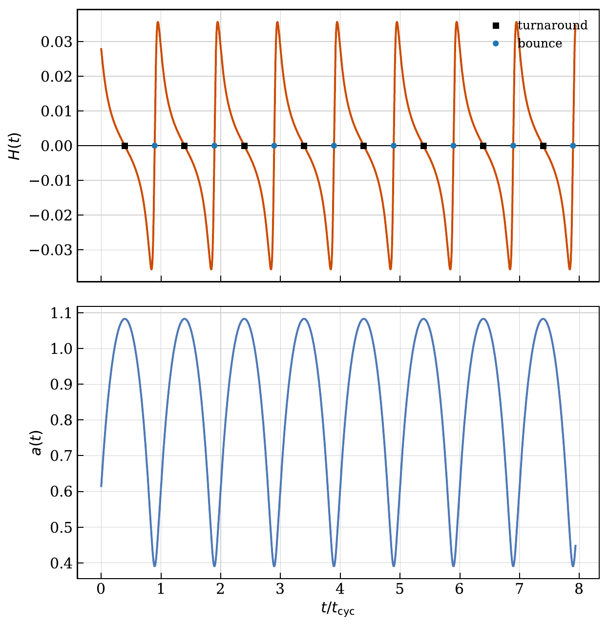
          <div className="title">Numerically integrated positively curved ECEM background</div>
        </div>
        <span className="meta"><M tex="k = +1" />{' '}representative run</span>
      </div>
      <div className="figure-body">
        <img
          className="journal-figure-img"
          src="assets/journal-figures/fig1-1.png"
          alt="Published Fig. 1 showing Hubble parameter and scale factor over multiple ECEM cycles"
        />
      </div>
      <div className="figure-caption">
        <strong>Fig. 1.</strong> A positively curved{' '}<M tex="k = +1" lead="(" tail=")" /> ECEM background integrated over multiple cycles. Closed spatial geometry allows the expansion to reverse at a classical turnaround{' '}<M tex="H = 0,\; \dot{H} < 0" lead="(" tail=")" /> without any torsion, while each subsequent contraction is halted by the spin–torsion bounce{' '}<M tex="H = 0,\; \dot{H} > 0" lead="(" tail=")." /> The top panel traces <M tex="H" /> alternating between these two types of zero crossing; the bottom shows the scale factor staying bounded and oscillatory rather than running into a singularity.
      </div>
    </section>
  );
}

// ============== Conceptual Cycle Diagram ==============
const CYCLE_PHASES = [
  {
    id: 'bounce',
    angle: 90,
    title: 'Torsion-supported bounce',
    short: 'Torsion Bounce',
    condTex: 'H = 0,\\;\\dfrac{dH}{dt} > 0',
    detail: <>
      As the universe contracts, the spin–torsion density{' '}<M tex="\rho_s \propto a^{-6}" />{' '}grows until it matches the total energy density. At that point the EC correction, which enters the Friedmann equation with a minus sign as{' '}<M tex="H^2 = (\rho_{\rm tot} - \rho_s)/3" />, forces{' '}<M tex="H^2" />{' '}to zero. Provided the equation of state has softened below{' '}<M tex="w = 1" tail="," /> the Raychaudhuri equation gives{' '}<M tex="\dot{H} > 0" />{' '}there, so{' '}<M tex="H" />{' '}crosses zero smoothly at a finite density{' '}<M tex="\rho_b" tail="." /> The bounce is obtained from the modified field equations rather than imposed as a cutoff.
    </>,
    color: 'var(--bounce)',
  },
  {
    id: 'expand',
    angle: 0,
    title: 'Scalar-dominated expansion',
    short: 'Scalar Expansion',
    condTex: 'w_\\varphi = \\dfrac{\\lambda^2}{3} - 1',
    detail: <>
      After the bounce the scalar sits on the positive plateau of the potential{' '}<M tex="V > 0" lead="(" tail=")" />{' '}with equation of state{' '}<M tex="w_\varphi = \lambda^2/3 - 1" tail="." /> The long-term dynamics are governed by the CLW attractor: for{' '}<M tex="\lambda^2 < 2" />{' '}the fixed point drives accelerated expansion; for{' '}<M tex="2 < \lambda^2 < 3\gamma_m" />{' '}it still attracts but without acceleration; above that the scalar and fluid scale together in a tracking solution.
    </>,
    color: 'var(--scalar)',
  },
  {
    id: 'matter',
    angle: 270,
    title: 'Matter / radiation era',
    short: 'Matter / Rad.',
    condTex: 'w_m = 0\\ \\text{or}\\ \\dfrac{1}{3}',
    detail: <>
      Between the bounce and ekpyrotic contraction sits a conventional fluid-dominated era. In the CLW variables{' '}<M tex="(x, y)" />, which measure the scalar's kinetic and potential energy fractions relative to the Hubble budget, the system idles near{' '}<M tex="(x,y) \approx (0,0)" />{' '}while matter or radiation carries the energy. This is a saddle in the full phase space: the trajectory passes through it rather than stopping there, eventually giving way to the scalar or to contraction.
    </>,
    color: 'var(--matter)',
  },
  {
    id: 'ekpyrosis',
    angle: 180,
    title: 'Ekpyrotic contraction',
    short: 'Ekpyrosis',
    condTex: 'w_\\varphi \\gg 1',
    detail: <>
      The scalar rolls down a steep negative branch of the potential, reaching{' '}<M tex="w_\varphi \gg 1" tail="," /> far stiffer than radiation. In this regime{' '}<M tex="\rho_\varphi \propto a^{-3(1+w_\varphi)}" />{' '}grows much faster during contraction than the shear{' '}<M tex="\rho_\sigma \propto a^{-6}" tail="," /> so the normalized shear{' '}<M tex="\Sigma = \sigma/H" />{' '}is driven exponentially toward zero. This is the key feature of ekpyrosis: whatever anisotropy the background starts with, the geometry is smoothed before the bounce.
    </>,
    color: 'var(--ekpyrotic)',
  },
];

function CycleDiagram() {
  const [active, setActive] = useStateI('bounce');
  const phase = CYCLE_PHASES.find(p => p.id === active);

  const cx = 250, cy = 220;
  const R = 130;
  const positions = CYCLE_PHASES.map(p => ({
    ...p,
    x: cx + R * Math.cos(p.angle * Math.PI / 180),
    y: cy - R * Math.sin(p.angle * Math.PI / 180),
  }));

  // Arc paths between neighboring phases, following the source order.
  const arcs = positions.map((p, i) => {
    const next = positions[(i + 1) % positions.length];
    // Curve each connector away from the center so the loop remains readable.
    const mx = (p.x + next.x) / 2, my = (p.y + next.y) / 2;
    // Unit normal pointing away from the center.
    const nx = (mx - cx) / Math.sqrt((mx - cx) ** 2 + (my - cy) ** 2);
    const ny = (my - cy) / Math.sqrt((mx - cx) ** 2 + (my - cy) ** 2);
    const cxC = mx + nx * 40;
    const cyC = my + ny * 40;
    return { from: p, to: next, cx: cxC, cy: cyC };
  });

  return (
    <div className="figure col-wide">
      <div className="figure-head">
        <div>
          <span className="label">Conceptual Guide</span>
          <div className="title">Four phases discussed in the ECEM model</div>
        </div>
        <span className="meta">Click any phase</span>
      </div>
      <div className="figure-body cycle-layout">
        <svg className="cycle-svg" viewBox="0 0 500 440" preserveAspectRatio="xMidYMid meet">
          {/* arrowhead def */}
          <defs>
            <marker id="arrow" viewBox="0 0 10 10" refX="9" refY="5" markerWidth="8" markerHeight="8" orient="auto">
              <path d="M0,0 L10,5 L0,10 Z" fill="var(--bounce)" />
            </marker>
          </defs>
          {/* arcs */}
          {arcs.map((a, i) => (
            <g key={'arc' + i}>
              <path
                d={`M ${a.from.x} ${a.from.y} Q ${a.cx} ${a.cy} ${a.to.x} ${a.to.y}`}
                fill="none"
                stroke="var(--bounce)"
                strokeWidth="2"
                strokeOpacity={active === a.from.id || active === a.to.id ? 1 : 0.5}
                markerEnd="url(#arrow)"
              />
            </g>
          ))}
          {/* central label */}
          <text x={cx} y={cy - 6} textAnchor="middle" fontSize="13" fill="var(--ink-soft)" fontFamily="var(--font-mono)" letterSpacing="0.15em">ECEM</text>
          <text x={cx} y={cy + 14} textAnchor="middle" fontSize="12" fill="var(--ink-faint)" fontFamily="var(--font-mono)">Cycle</text>
          {/* nodes */}
          {positions.map(p => {
            const isActive = active === p.id;
            return (
              <g key={p.id} className={'cycle-node ' + (isActive ? 'active' : '')}
                onClick={() => setActive(p.id)}>
                <foreignObject x={p.x - 85} y={p.y - 26} width={170} height={56}>
                  <div xmlns="http://www.w3.org/1999/xhtml"
                    className={'cycle-node-box ' + (isActive ? 'active' : '')}>
                    <div className="cycle-node-title">{p.short}</div>
                    <div className="cycle-node-cond"><M tex={p.condTex} /></div>
                  </div>
                </foreignObject>
              </g>
            );
          })}
        </svg>
        <div>
          <div className="tag-pill bounce">{phase.id.toUpperCase()}</div>
          <h3 style={{ marginTop: 14, marginBottom: 8 }}>{phase.title}</h3>
          <div className="mono" style={{ color: 'var(--ink-soft)', marginBottom: 12, fontSize: 13 }}><M tex={phase.condTex} /></div>
          <p style={{ fontSize: 15, color: 'var(--ink-mid)', lineHeight: 1.55, marginBottom: 0 }}>{phase.detail}</p>
        </div>
      </div>
      <div className="figure-caption">
        <strong>Conceptual guide.</strong> Not a journal figure, but a map of the four dynamical regimes discussed in the paper. The published Fig. 1 above shows a numerically integrated{' '}<M tex="k = +1" />{' '}trajectory cycling through these phases. Click any node to read what is happening physically at that stage.
      </div>
    </div>
  );
}

Object.assign(window, { Hero, Abstract, PublishedFig1, CycleDiagram });
